API

Getting started

You can utilize DAVe modules throught the `dave.ocpu.client` package. All DAVe functionality not listed below can be implemented using the module `R` libraries directly.

Follow the installation instructions before trying the examples below.

Connect to API endpoints

The following examples all use opencpu servers to enable calculations. Check the opencpu documentation for more details.

Code

library(dave.ocpu.client)
source(system.file('app/src/API.R',package='dave.app'))

Check connections

Code

library(dplyr)
apis <- c(
  'dave.ml' = dave_ml_connection,
  'ctsgetr' = ctsgetr_connection,
  'dave.network' = dave_network_connection,
  'dave.path' = dave_path_connection,
  'dave.multivariate' = dave_multivariate_connection
)

lapply(1:length(apis), function(i){

  status<-apis[[i]]$get()$status_code ==200

  data.frame(endpoint=names(apis)[i], status = ifelse(status,'OK','DOWN'))


}) %>%
  do.call('rbind',.)

           endpoint status
1           dave.ml     OK
2           ctsgetr     OK
3      dave.network     OK
4         dave.path     OK
5 dave.multivariate     OK

Multivariate analysis

Carry out principal components analysis (PCA). Get more details about the implemented PCA methods.

Before following the examples below, first connect to the API endpoints as shown above.

View all available PCA methods

Code

x<-ocpu_dvmPCA_methods(dave_multivariate_connection)

No encoding supplied: defaulting to UTF-8.

Code

x$results

 [1] "svd"          "nipals"       "rnipals"      "bpca"         "ppca"        
 [6] "svdImpute"    "robustPca"    "nlpca"        "llsImpute"    "llsImputeAll"

Load demo data

Code

library(dave.multivariate.app)
data("dave_data")
data<-dave_data

Calculate PCA

Code

body <- list(
  data=data,
  pca.components = 2,
  pca.cv = 'q2',
  pca.algorithm = "svd",
  pca.center = TRUE,
  pca.scaling = "uv",
  seed = 123,
  return = "list"
)

x<-ocpu_dvmPCA(dave_multivariate_connection,body=body)
.pca<-x$results

Get PCA summary

Code

summary(.pca)$description

[1] "Principal components analysis was conducted using the svd method. The data set was centered and scaled using uv. A total of 2 components were calculated, explaining 28.2% variance in the data set. The cross-validated variance explained was 36.1%."

Plot

Specify metadata for all plots

Code

data("dave_data_row_meta")
color<-dave_data_row_meta %>% select(class)
label<-dave_data_row_meta %>% select(label)
plot_args<-list(size=5,labels=label,color=color,label=TRUE)

Eigenvalues scree scores

Code

# plot_args$type<-'scree'
p<-plot(.pca,plot_args=plot_args,plot_type='scree')
plotly::ggplotly(p)

Warning: `gather_()` was deprecated in tidyr 1.2.0.
ℹ Please use `gather()` instead.
ℹ The deprecated feature was likely used in the plotly package.
  Please report the issue at <https://github.com/plotly/plotly.R/issues>.

Eigenvalues cummulative plot

Code

plot_args$type<-'cumm'
p<-plot(.pca,plot_type='cumm',plot_args=plot_args) #type not changing
# p<-dave.multivariate.app:::dvmPCA_scree_plot(.pca, type='cumm')
plotly::ggplotly(p)

Sample scores plot

Code

plot_args$type<-NULL
plot_args$point.labels<-plot_args$labels
plot_args$font.size<-3
p<-plot(.pca,plot_type='scores',plot_args=plot_args) #
plotly::ggplotly(p)

Sample outlier diagnostics plot

Code

plot_args$type<-NULL
plot_args$point.labels<-plot_args$labels
plot_args$font.size<-3
p<-plot(.pca,plot_type='diagnostic',plot_args=plot_args) #
plotly::ggplotly(p)

Variable loadings plot

Code

data("dave_data_col_meta")
plot_args$color<-NULL
plot_args$point.labels<-dave_data_col_meta$name
plot_args$font.size<-2
p<-plot(.pca,plot_type='loadings',plot_args=plot_args) #
plotly::ggplotly(p)

Scores and loadings biplot

Code

data("dave_data_col_meta")
plot_args$color<-dave_data_row_meta %>% select(class)
plot_args$point.labels<-dave_data_col_meta$name
plot_args$font.size<-2
p<-plot(.pca,plot_type='biplot',plot_args=plot_args) #
plotly::ggplotly(p)

Machine learning

Before following the examples below, first connect to the API endpoints as shown above.

Train machine learning models

Load sample data

Code

library(dave.stat)
library(dave.ml.app)

data("dave_data")
tmp<-dave_data
y<-'class'
.y<-dave_data_row_meta$class
tmp[y]<-.y

Specify tuning and performance metrics

Code

.metric<-'Kappa'
.method<-c('rf')
classProbs<-TRUE
tuneN<-1
tuneGrid<-NULL

Create model train and test data

Code

body<-list(data=tmp,y=y)
.data<-ocpu_create_model_data(dave_ml_connection ,body=body)

Define model cross validation

Code

body<-list(method="repeatedcv",num=7,rep=3,classProbs=classProbs)  #this need to be flattened to a string
fitControl <- ocpu_create_fit_control(dave_ml_connection ,body=body)

Train selected model

Code

# create model
body <-
  list(
    data = .data,
    y = y,
    metric = .metric,
    method = .method,
    fitControl = fitControl,
    tuneN = tuneN,
    tuneGrid = tuneGrid,
    seed= 1234
  )

mod<-ocpu_multi_create_predictive_model(dave_ml_connection ,body = body)

Get model performace summary

Code

body<-list(multi_mod=mod)
ocpu_get_model_perf(dave_ml_connection ,body=body)

$meta $meta$session [1] “x0ab7c097aceeee”

$meta$status [1] 201

$paths [1] “/ocpu/tmp/x0ab7c097aceeee/R/.ocpu_get_model_perf” “/ocpu/tmp/x0ab7c097aceeee/R/.val” “/ocpu/tmp/x0ab7c097aceeee/stdout”
[4] “/ocpu/tmp/x0ab7c097aceeee/source” “/ocpu/tmp/x0ab7c097aceeee/console” “/ocpu/tmp/x0ab7c097aceeee/info”
[7] “/ocpu/tmp/x0ab7c097aceeee/files/DESCRIPTION”

$results $results$description [1] “Machine learning based predictive modelling was used to predict class. A single model was fit and optimized based on predictive performance on the test data.A random forest model was developed on 51 samples and 188 predictors to predict 2 classes: diabetic.., non.diabetic.. with no pre-processing. Cross validation was done by resampling: cross-validated (7 fold, repeated 3 times) . Tuning parameter ‘mtry’ was held constant at a value of 62.”

$results$table model train test metric maximize time_min 1 rf 0.6173153 0.7148289 Kappa TRUE 0.04736702

$results$best model train test metric maximize time_min 1 rf 0.6173153 0.7148289 Kappa TRUE 0.04736702 description 1 A random forest model was developed on 51 samples and 188 predictors to predict 2 classes: diabetic.., non.diabetic.. with no pre-processing. Cross validation was done by resampling: cross-validated (7 fold, repeated 3 times) . Tuning parameter ‘mtry’ was held constant at a value of 62.

Plot model results

Code

library(dave.ml.app)
.mod<-get_ocpu_obj(ocpu_session(mod),dave_ml_connection$url)
x<-dave.ml.app::plot.model_list(.mod,type='model',print=FALSE) 
ggplotly(x)

Code

# see other types c('performance', 'model','importance','confusion','classification')

Code

library(dave.ml.app)
.mod<-get_ocpu_obj(ocpu_session(mod),dave_ml_connection$url)
x<-dave.ml.app::plot.model_list(.mod,type='classification',curve='pr',print=FALSE) 
ggplotly(x)

Code

library(dave.ml.app)
.mod<-get_ocpu_obj(ocpu_session(mod),dave_ml_connection$url)
x<-dave.ml.app::plot.model_list(.mod,type='confusion',percent=FALSE,print=FALSE) 
x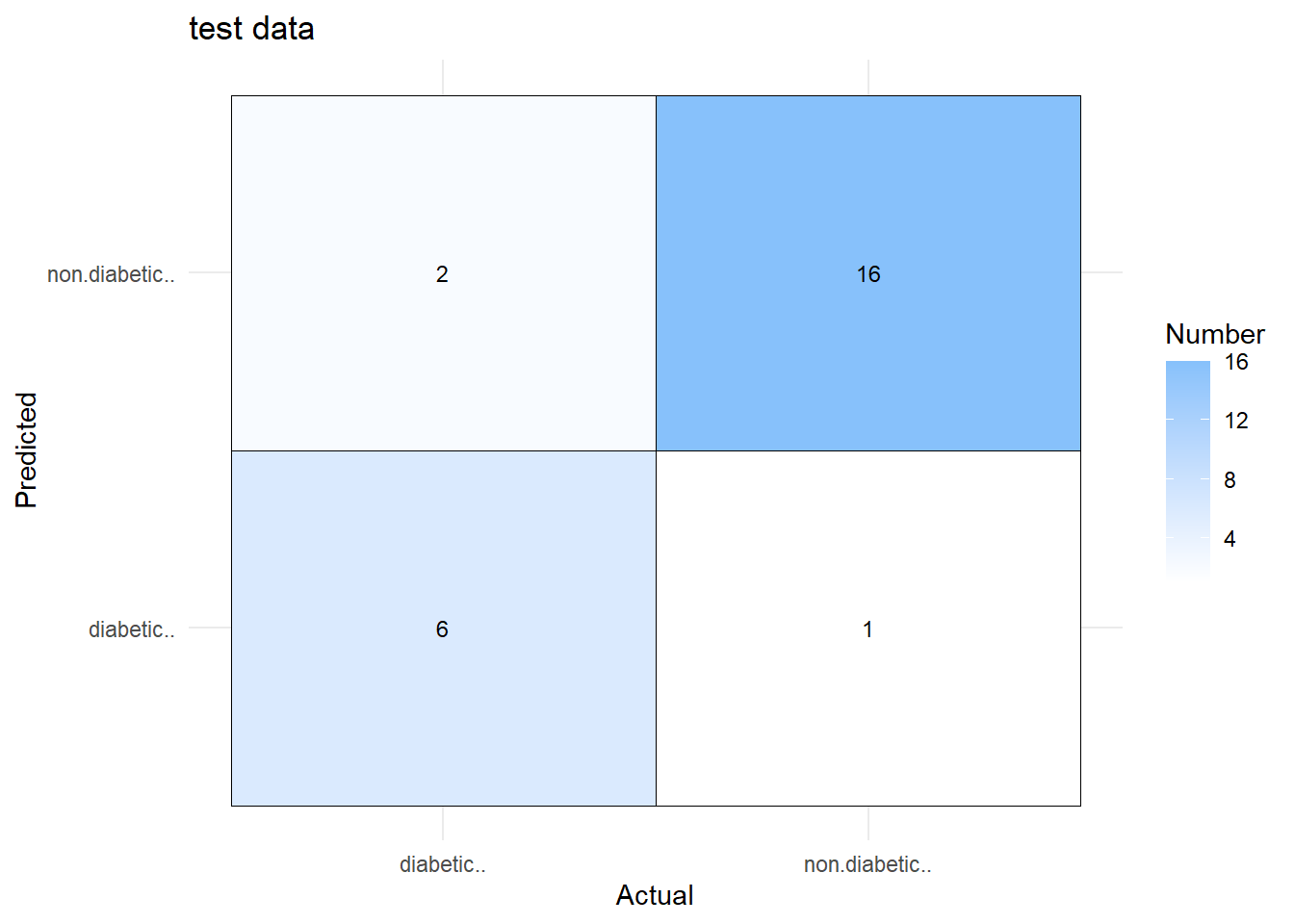

Code

# ggplotly(x) # see other types c('performance', 'model','importance','confusion','classification')

Feature selection

Use recursive feature elimination `RFE` to reduce model features (variables) and increase model performance.

Specify RFE options

Code

func<-'rfFuncs' # randomforest
repeats<-1 # repeated CV
number<-5 # CV folds
body<-list(func=func,repeats=repeats,number=number)
ctrl<-ocpu_create_rfe_control(dave_ml_connection ,body)

Specify hyperparameters tuning and

Code

# Increase 'tuneLength' to add more tuning hyperparameter tune grid combinations.
tuneLength<-1
seed<-123

# Specify training data
body<-list(obj=.data,
           name='train.data')

train_data<-get_ocpu_list_item(dave_ml_connection ,body)

#specify variable subsets for RFE
#NOTE: referencing previous ocpu session objects dynamically in ocpu calls is not easy. If we need to create a subset for RFE we need to calculate this object in another session and reference its results. To do this we also need to calculate the total number of columns in the `train_data`.

#get total number of columns/features in the data
#encode NULL is used to reference the session. The encoding = 'form' can be used for more complex requirements. 
body <- list(x = ocpu_session(train_data))
pkg_url <-  'ocpu/library/base/R/dim'

dims<-ocpu_post(
  dave_ml_connection,
  body = body,
  pkg_url = pkg_url,
  encode = NULL,
  return_value = TRUE
)$results


#create subset
body <- list(from=1,to=dims[2],by=3)
pkg_url <-  'ocpu/library/base/R/seq'
return_value <- FALSE

.subset<-ocpu_post(
  dave_ml_connection,
  body = body,
  pkg_url = pkg_url,
  encode = 'json',
  return_value = return_value
)

#carry out RFE feature selection
body <-
  list(data = train_data,
        y = y,
       subset = .subset,
       ctrl = ctrl,
       tuneLength = tuneLength,
       seed = seed)


rfe<-ocpu_create_rfe(dave_ml_connection ,body)

Select best variables

Code

#pick subset
best<- 'PickSizeBest' #'pickSizeTolerance' #"PickSizeBest"#'pickSizeTolerance'
metric<-'Kappa'
body<-list(rfRFE=rfe,best=best, metric=metric,tolerance=.1)

# best<- 'pickSizeTolerance'
# tolerance<-5
# body<-list(rfRFE=rfe,best=best,tolerance=tolerance)


#get top model variables
selected_rfe<-ocpu_rebuild_rfe(dave_ml_connection ,body)
.selected_rfe<-get_ocpu_obj(ocpu_session(selected_rfe),dave_ml_connection$url)

Model summary

Code

library(dave.ml.app)
#collect all required args
rfe_select_args<-list(
  best_subset = best,
  metric = metric,
  tolerance = NULL,
  func = func
)

do.call('summary.model_rfe',list(c(.selected_rfe,rfe_select_args)))

[1] "Recursive feature elimination (RFE) was used to identify top predictive variables. Backward and forward variable selection was done to optimize model Kappa using rfFuncs, validated with  for  folds repeated  times while conducting  round(s) of model parameter tuning. The final model was selected based on the best subset method. The selected model contains 16 variable(s) and has Kappa equal to 0.701 +/- 0.163. The top 5 variables include: var188, var173, var51, var15 and var34."

Plot results

Code

x<-dave.ml.app::plot.model_rfe(.selected_rfe,metric = metric,print=FALSE) 
ggplotly(x)

Metabolite identifier translation

Translate metabolite identifiers between > 200 of the most common databases.

Before following the examples below, first connect to the API endpoints as shown above.

Demo data

Code

trans_args<-function(){list(url = "http://ec2-107-21-83-113.compute-1.amazonaws.com:81/ocpu/", body = list(
  id = c("C00310", "C00379", "C01762", "C00385", "C00183", 
         "C02067", "C00299", "C00366", "C00086", "C00106", "C00082", 
         "C00078", "", "C06771", "C01083", "C01157", "C02477", "C00178", 
         "C00214", "C00188", "", "", "C00245", "D09007", "C00059", 
         "C00089", "C00042", "C01530", "C00794", "C08250", "C00493", 
         "C00065", "C00213", "C00818", "C00199", "C00121", "C00474", 
         "C00507", "C00022", "C00013", "", "C02457", "C00148", "", 
         "C00009", "C00346", "", "C00079", "C07086", "C01601", "C00864", 
         "C08362", "C00249", "C01879", "C00209", "C00295", "C00077", 
         "C00712", "C02721", "C00253", "C00153", "", "", "C00624", 
         "", "C00645", "C03136", "", "C02989", "C00073", "", "", "C00208", 
         "C00149", "C07272", "", "C00047", "C06427", "C01595", "C01725", 
         "", "C02679 ", "", "C00186", "C00328", "", "C00407", "C00311", 
         "", "", "C00294", "C02043", "C00954", "C16526", "C00262", 
         "C00192", "", "C05629", "C00263", "C01817", "C00135", "", 
         "C00387", "C00160", "C00037", "C00093", "C05401", "C00258", 
         "C00489", "C00064", "C00025", "C00191", "C00092", "C00031", 
         "C00257", "", "C00446", "C00124", "C00880", "C01235", "C00122", 
         "C01018", "C01019", "C00085", "C00095", "C00189", "C00503", 
         "C08374", "", "C00112", "", "C00097", "C00791", "", "C00327", 
         "C00158", "C00695", "C00187", "", "C06423", "C01571", "C03044", 
         "C00099", "C00180", "C08281", "C00049", "C00152", "", "C06425", 
         "C01904", "C00259", "C00872", "C00026", "C01551", "C00499", 
         "C00041", "C06104", "C00020", "C00212", "C00417", "C05659", 
         "", "C01015", "C07588", "C00989", "C00156", "", "C00197", 
         "", "C01013", "C01089", "", "C06474", "", "C00629", "C02112", 
         "C00233", "", "C02630", "C05984", "", "", "C00956", "", "D01947", 
         "", "C01885", "C07326"), from = "KEGG", to = c("KEGG", "InChIKey"
         ), db_name = "/ctsgetr/inst/ctsgetr.sqlite", from_obj = "KEGG"))}

Code

body<-trans_args()$body

x<-ocpu_post(
  ctsgetr_connection,
  body = body,
  pkg_url = 'ocpu/library/CTSgetR/R/CTSgetR',
  encode = 'json',
  return_value = TRUE
)

No encoding supplied: defaulting to UTF-8.

Code

head(x$results)

      id                    InChIKey   KEGG
1 C00310 LQXVFWRQNMEDEE-OVEKKEMJSA-N C00310
2 C00379 HEBKCHPVOIAQTA-SCDXWVJYSA-N C00379
3 C01762 UBORTCNDUKBEOP-UUOKFMHZSA-N C01762
4 C00385 LRFVTYWOQMYALW-UHFFFAOYSA-N C00385
5 C00183 KZSNJWFQEVHDMF-BYPYZUCNSA-N C00183
6 C02067 PTJWIQPHWPFNBW-GBNDHIKLSA-N C02067

Network analysis

Calculate emprical regularized correlation, biochemical relationships and structural similarity networks. Each module supports rich static, interactive and dynamic network visualizations.

Get more details.

Before following the examples below, first connect to the API endpoints as shown above.

The following will show how to calculate various networks. See the visualize neyworks section below for network plotting examples. Note,a ll of the edge lists are indexed on `dave_network_col_meta$id`, see `dave_network_col_meta` to view the corresponding molecule names.

Load demo data

Code

library(dave.network.app)
data("dave_network")
data("dave_network_col_meta")
data<-dave_network_col_meta

Chemical similarity

The following is an example of how to calculate Tanimoto similarity based on molecule PubChem chemical identifiers fingerprints.

Code

idcolumn<-'CID'
net_index<-'id'
type<-'CID'
DB <- '/open_cpu/CID.SDF.DB'


body<-list(data=data,
           idcolumn=idcolumn,
           type = type,
           net_index = net_index,
           DB=DB)

net <- structural_net <-
  ocpu_metabolic_network(dave_network_connection, body = body,return_value = TRUE)

lapply(net$results,head)

$nodes
    ID       name   KEGG     CID id
1 var1   xylulose C00310 5289590  1
2 var2    xylitol C00379    6912  2
3 var3 xanthosine C01762   64959  3
4 var4   xanthine C00385    1188  4
5 var5     valine C00183    6287  5
6 var6    uridine C02067   15047  6

$edges
    from to     value   value.1 type
176  153 27 0.7027027 0.7027027  CID
351  153 74 0.6304348 0.6304348  CID
352   27 74 0.6923077 0.6923077  CID
526  153 39 0.6486486 0.6486486  CID
527   27 39 0.6250000 0.6250000  CID
528   74 39 0.5609756 0.5609756  CID

$node_mapping
NULL

$vis_config
NULL

Biochemical relationships

The following example shows how to calculate molecule reactions precursor to product relationships based on KEGG identifiers.

Code

idcolumn<-'KEGG'
net_index<-'id'
type<-'KEGG'
DB <- '/open_cpu/CID.SDF.DB'


body<-list(data=data,
           idcolumn=idcolumn,
           type = type,
           net_index = net_index,
           DB=DB)

net <- biochem_net<-
  ocpu_metabolic_network(dave_network_connection, body = body)

lapply(net$results,head)

$nodes
    ID       name   KEGG     CID id
1 var1   xylulose C00310 5289590  1
2 var2    xylitol C00379    6912  2
3 var3 xanthosine C01762   64959  3
4 var4   xanthine C00385    1188  4
5 var5     valine C00183    6287  5
6 var6    uridine C02067   15047  6

$edges
  from  to value value.1 type
1    1   2     1       1 KEGG
2    1 150     1       1 KEGG
3    4   3     1       1 KEGG
4   36   3     1       1 KEGG
5  103   3     1       1 KEGG
6   95   4     1       1 KEGG

$node_mapping
NULL

$vis_config
NULL

Regularized correlations

The following example shows how to calculate and regularize empirical correlation relationships among any numeric data.

Code

library(dave.network.app)

data("dave_network")
tmp_data<-dave_network

Calculate correlations

Code

body <- list(
  data = tmp_data,
  cor_method = 'spearman',
  cor_FDR = TRUE,
  cor_cutoff = .05,
  lambda = NULL,
  huge_method = 'manual'
)

x <-
  ocpu_get_cor_mat(dave_network_connection,
                   body = body)

Regularize network

Code

body <-
  list(
    data = tmp_data,
    nlambda = 10,
    paranorm = TRUE,
    lambda.min.ratio = .1,
    check.cor = FALSE
  )


huge_obj<-
  ocpu_get_huge_obj(dave_network_connection,
                      body = body,
                    return_value = TRUE)

Select top relationships

Note, you can also use `opt=maual` and specify a `lambda` to manualy tune the network connection strength.

Code

body <-
  list(
    huge_obj=huge_obj,
    lambda=NULL, #round(huge_obj$results$lambda[5],4), # legacy shenanigans for manual
    opt='stars'
  )

huge_edges<-
  ocpu_get_huge_edges(dave_network_connection,
                    body = body)

head(huge_edges$results)

  source target value
1      2      1     1
2     24      1     1
3     30      1     1
4     36      1     1
5     39      1     1
6     79      1     1

Visualize networks

Code

#load calculated objects for the network nodes
library(dave.stat)
data("dave_stat_col_meta")

#join external analysis results with a calculated network
network_obj <- biochem_net$results

#match internal indicies
dave_stat_col_meta$id <- gsub('var', '', dave_stat_col_meta$ID)

network_obj$nodes <-
  left_join(network_obj$nodes, dave_stat_col_meta, by = 'id')

#create mappings for node attributes
FC <-
  map_fold_change(network_obj$nodes$FC_non.diabetic.._diabetic.., transform = 'log2')$results


FC$'_dir' <- factor(FC$'_dir',labels = c('increased','unchanged','decreased'),levels = c(1,0,-1))



network_obj$nodes <- cbind(network_obj$nodes, FC = FC)


network_obj$node_mapping <- list(
  node_col = 'FC._dir',
  node_size = 'FC._mag',
  node_label = 'name.y',
  node_size_range = c(3, 7)
)

x <- do.call('network.visualize', network_obj)


# network.visnetwork(x)
ggplotly(dave.network.app:::plot.network_viz(x))

Debug API calls

Code

library(dave.ocpu.client)
source(system.file('app/src/API.R',package='dave.app'))

This section shows examples how to debug and determine what might be going wrong when an API call fails.

Execute a remote calculation. Lets do something simple like get the column names of a local data set. This will show how to make a request and get the results. In practice, `DAVe` API endpoints only require a `body` argument and you can see all the created asset paths by setting `return_value = FALSE`.

Code

data("mtcars")

body<-list(x=mtcars)
pkg_url <-  'ocpu/library/base/R/colnames' #this will call base::colnames

res0<-ocpu_post(
  dave_ml_connection,
  body = body,
  pkg_url = pkg_url,
  encode = 'json',
  return_value = TRUE
)$results

res0

 [1] "mpg"  "cyl"  "disp" "hp"   "drat" "wt"   "qsec" "vs"   "am"   "gear" "carb"

Make a request and view the created assets without retrieving the results.

Code

res1<-ocpu_post(
  dave_ml_connection,
  body = body,
  pkg_url = pkg_url,
  encode = 'json',
  return_value = FALSE
)

cat('Add the "$paths" below to the following url to view the results:')

Add the "$paths" below to the following url to view the results:

Code

cat(dave_ml_connection$url)

http://ec2-52-22-43-130.compute-1.amazonaws.com/ml/

Code

res1

$meta
$meta$session
[1] "x059dd61ae4576c"

$meta$status
[1] 201


$paths
[1] "/ocpu/tmp/x059dd61ae4576c/R/.val"            "/ocpu/tmp/x059dd61ae4576c/R/colnames"        "/ocpu/tmp/x059dd61ae4576c/R/x"               "/ocpu/tmp/x059dd61ae4576c/stdout"           
[5] "/ocpu/tmp/x059dd61ae4576c/source"            "/ocpu/tmp/x059dd61ae4576c/console"           "/ocpu/tmp/x059dd61ae4576c/info"              "/ocpu/tmp/x059dd61ae4576c/files/DESCRIPTION"

Get the created object from a previous call

Code

get_ocpu_obj(ocpu_session(res1) ,dave_ml_connection$url)

 [1] "mpg"  "cyl"  "disp" "hp"   "drat" "wt"   "qsec" "vs"   "am"   "gear" "carb"

Reference the previous request’s results in another calculation.

Code

body<-list(x=res1, collapse='|')
pkg_url <-  'ocpu/library/base/R/paste' 

ocpu_post(
  dave_ml_connection,
  body = body,
  pkg_url = pkg_url,
  encode = 'form',
  return_value = TRUE
) $results

[1] "mpg|cyl|disp|hp|drat|wt|qsec|vs|am|gear|carb"

You can include multiple session’s results to execute more complicated calculations. The example below shows how to get the row and column names of the data and then create a sequence based on the total number of rows. The function `ocpuclient::get_ocpu_list_item` is useful for selecting specific named list elements from previous sessions results.

Code

#get a specific element from a previous session either by list index or name
body<-list(obj='<NAME of OBJECT>',
           name='<NAME of LIST ITEM>')

get_ocpu_list_item(dave_ml_connection ,body)

Getting started

You can utilize DAVe modules throught the dave.ocpu.client package. All DAVe functionality not listed below can be implemented using the module R libraries directly.

Follow the installation instructions before trying the examples below.

Connect to API endpoints

The following examples all use opencpu servers to enable calculations. Check the opencpu documentation for more details.

Check connections

Multivariate analysis

Carry out principal components analysis (PCA). Get more details about the implemented PCA methods.

Before following the examples below, first connect to the API endpoints as shown above.

View all available PCA methods

Load demo data

Calculate PCA

Get PCA summary

Plot

Specify metadata for all plots

Eigenvalues scree scores

Eigenvalues cummulative plot

Sample scores plot

Sample outlier diagnostics plot

Variable loadings plot

Scores and loadings biplot

Machine learning

Before following the examples below, first connect to the API endpoints as shown above.

Train machine learning models

Load sample data

Specify tuning and performance metrics

Create model train and test data

Define model cross validation

Train selected model

Get model performace summary

Plot model results

Feature selection

Use recursive feature elimination RFE to reduce model features (variables) and increase model performance.

Specify RFE options

Specify hyperparameters tuning and

Select best variables

Model summary

Plot results

Metabolite identifier translation

Translate metabolite identifiers between > 200 of the most common databases.

Before following the examples below, first connect to the API endpoints as shown above.

Demo data

Network analysis

Calculate emprical regularized correlation, biochemical relationships and structural similarity networks. Each module supports rich static, interactive and dynamic network visualizations.

Get more details.

Before following the examples below, first connect to the API endpoints as shown above.

The following will show how to calculate various networks. See the visualize neyworks section below for network plotting examples. Note,a ll of the edge lists are indexed on dave_network_col_meta$id, see dave_network_col_meta to view the corresponding molecule names.

Load demo data

Chemical similarity

The following is an example of how to calculate Tanimoto similarity based on molecule PubChem chemical identifiers fingerprints.

Biochemical relationships

The following example shows how to calculate molecule reactions precursor to product relationships based on KEGG identifiers.

Regularized correlations

The following example shows how to calculate and regularize empirical correlation relationships among any numeric data.

Calculate correlations

Regularize network

Select top relationships

Note, you can also use opt=maual and specify a lambda to manualy tune the network connection strength.

Visualize networks

Debug API calls

This section shows examples how to debug and determine what might be going wrong when an API call fails.

Execute a remote calculation. Lets do something simple like get the column names of a local data set. This will show how to make a request and get the results. In practice, DAVe API endpoints only require a body argument and you can see all the created asset paths by setting return_value = FALSE.

Make a request and view the created assets without retrieving the results.

Get the created object from a previous call

Reference the previous request’s results in another calculation.

You can utilize DAVe modules throught the `dave.ocpu.client` package. All DAVe functionality not listed below can be implemented using the module `R` libraries directly.

Use recursive feature elimination `RFE` to reduce model features (variables) and increase model performance.

The following will show how to calculate various networks. See the visualize neyworks section below for network plotting examples. Note,a ll of the edge lists are indexed on `dave_network_col_meta$id`, see `dave_network_col_meta` to view the corresponding molecule names.

Note, you can also use `opt=maual` and specify a `lambda` to manualy tune the network connection strength.